Hi All!! today I will be writing about another piece of research I completed as part of my PhD. The premise of this work revolves around explainable-AI, specifically in the domain of cybersecurity. In recent years there has been an increasing effort of utilizing Machine Learning and Deep Learning models for cybersecurity applications, ranging from intrusion detection to malware classification.
However, most of these state-of-the-art deep learning models are treated as black-boxes, meaning that we aren’t able to explain why a given model predicts some malicious activity, which makes it hard for an analyst or threat hunter to identify if an alert is truly malicious. To circumvent this issue there has been a growing interest in explaining deep learning models used for cybersecurity tasks.

In my PhD work we pushed the boundary in explaining deep-learning based malware classification by introducing an explainer named CFGExplainer (paper, code). Graph Neural Networks have shown great promise in malware classification tasks, where the malware source code is processed and presented in a graph format called an Attributed Control Flow Graph (ACFG). However, explaining how these detections work is hard, mainly because a given malware graph can have over thousands of nodes and edges. Identifying which exact portion of the graph (i.e., subgraph) represents malicious code while pruning out the less important bits efficiently is the main challenge addressed in this work.
Malware classification with GNNs
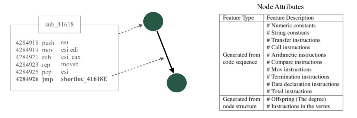
In this first section, I will go through a brief overview of how source code is converted to a graph format for our detection task. Typically, in an Attributed Control Flow Graph nodes represent basic blocks of code that have atomic executions as shown in the image above. The edges between these basic blocks are the connectivity through call, jump instructions or of how the code flows through from one block to another. For each node, we define node features based on the type of instructions present within the code block.
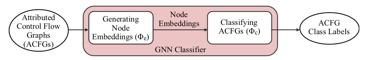
After this step, the graphs are processed by a Graph Neural Network (GNN) model. A GNN model usually operates in two stages. First it processes the node/edge features and the spatial connectivity in the graph to produce node embeddings. These node embeddings are latent representations of nodes that capture information useful for some subsequent task, in our case the node embeddings contain important information with respect to malware classification. Then in the next stage the node embeddings are processed by a feed forwarding neural network that produces classification probabilities based on the malware types.
CFGExplainer
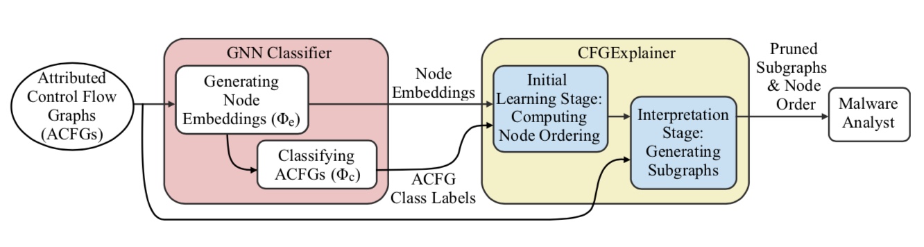
The figure above shows the architecture of our solution. In our work, we assume that there exists some GNN model that is capable of classifying attributed control flow graphs into their respective malware types. Initially the graph samples to be explained are processed by the GNN classifier, which produces both the node embeddings and the malware class labels. Then these embeddings, labels and the original graphs are provided to CFGExplainer.
CFGExplainer operates in two stages. First in an initial learning stage, the explainer learns to score nodes with respect to their contribution towards malware classification. Then in the second stage the explainer prunes out nodes that have the least importance. This pruned subgraph is provided as an explanation to the analyst along with an ordering of nodes based on importance to classification.
The learning stage is carried out through two interconnected neural network components (a node scoring module and a surrogate classifier) that are jointly trained to identify important nodes.
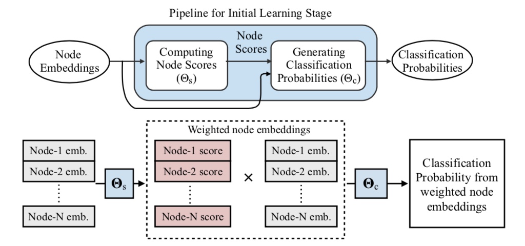
In the forward pass in this algorithm,
- First the node embeddings are processed and a score is produced for each embedding. Here a larger score correspond to the node being viewed as more important.
- Then the scores are multiplied against the original node embeddings to produce a weighted node embedding per node.
- Finally, these weighted node embeddings are fed through a second neural network module (i.e., a surrogate classifier) that produces classification probabilities for the malware families.
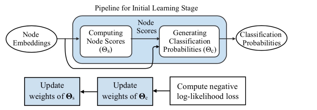
After producing the classification probabilities, the backward pass is carried out as a back-propagation step where the objective is to mimic the malware detection capability of the original GNN model through this surrogate classifier using weighted node embeddings. Notice that due to this joint training, as the surrogate classifier learns to better mimic the original GNN, the node scoring module learns to produce higher scores for more important nodes.
Once this training is completed using all the graphs to be explained, the explainer can directly prune out nodes with smaller scores, leaving a subgraph that contributes most towards the malware classification task.
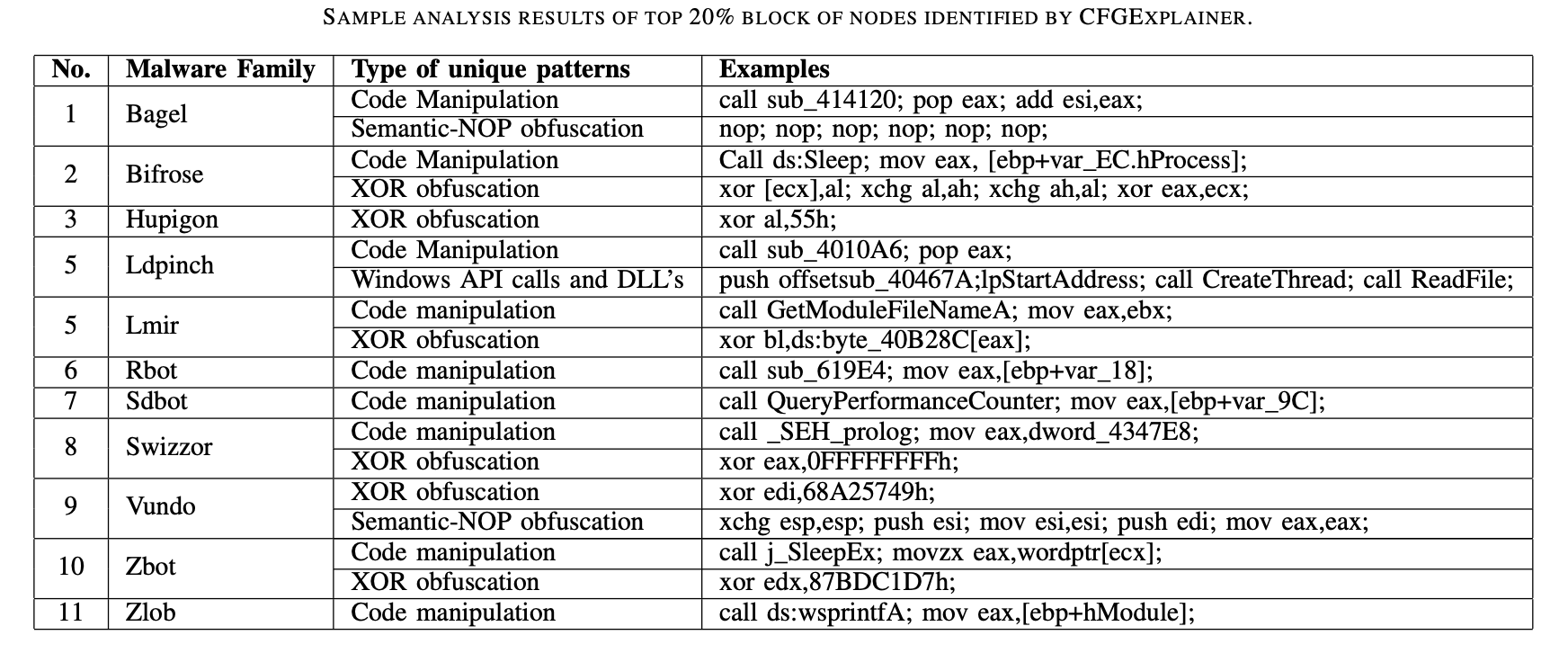
In our experiments we found that CFGExplainer is able to produce subgraphs (~20% original size) that indicate malicious patterns such as obfuscation tricks and code manipulations that would have been harder to manually identify by analyzing the complete malware graph. If you want to learn more about CFGExplainer please check our paper and code.