Hi All! Today I thought of writing an introductory post on implementing Deep Learning models using Tensorflow. In recent years you probably have heard about AI beating players in quite complex games like GO and DOTA and probably thought it’s really cool. This explosive development in machine intelligence is due to advancements in Deep Learning, which is a branch of machine learning that extends from neural networks.
Deep Learning has been used in many application domains from image and video processing to time series forecasting and creating autonomous agents that could say play games. Now, to be very specific I will be talking about a subset of deep learning models that are specifically designed to work with time series data. Referring to the image up top these models can be grouped together into what’s called Recurrent Neural Networks (RNN). These are a set models that have the capability to identify temporal correlation in data.
To clarify, my post today will not be about explaining how a recurrent neural network works, instead I will walk you through snippets of code that will help you to build your own RNN model. So I am assuming you know somewhat about how RNNs work and the theory behind it and have some understanding about Tensorflow. If you don’t know much about deep learning and RNNs these links below are good places to start learning about these models.
- The set of free Deep Learning course by Cognitive Class.
- Free Deep Learning course by Udacity.
- The online version of deeplearningbook.
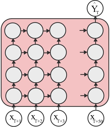
The RNN I will be explaining today takes in sequences of 50 (T+1 to T+50 where T is the time step) times series values to the immediate past and predicts the future variation based on it. This kind of RNN can be used to predict variations in temperature, humidity, ran fall, signal strength ect. For clarity, I will break down my post into three sections. In Part 1 I will talk about data preprocessing, namely how I convert a univariate time series (i.e. the time series has only one feature) into an appropriate input format to the model. In Part 2 I will talk about the model itself and finally in Part 3 I will present the code to run the model.
Part 1 : Data Preprocessing
Data preprocessing is a very important part in many Machine learning applications. And more often than not, the most important part of applying models is to understand the data so that you know to pick the best model for your data. Once you pick the model, the data needs to be preprocessed in a way the model understands it. For this example, referring to the image above the model takes in sequences of data. Let’s say we have a time series of 1000 values [1,2,3,…,999,1000]. The RNN model needs input as sequences of data where the model will learn the temporal behavior of each sequence. In this case if say the sequence length is 50, then the model needs sequences [1-50],[2-51],[3-52]… with unit time step for all the data.
The function getData converts a list of univariate time series values into a sequences of data used for both training and testing the model. The input parameters are the filename use to load data, the x_length the size of the input sequence (as per the figure default is 50), the y_length the number of future predictions made by the RNN and finally the percentage between training and test data separation. Usually and 80:20 split for training:testing is used in most models so percentage=0.8 usually works. This function returns the sequences used for training and testing and the predictor labels as well. The helper functions openFile and sampleData used within getData reads data from file and creates the sequences respectively. I usually create a separate python file DataPreprocessor.py and use the functions herewith to preprocess the input data.
""" Main Function to preprocess dataset --------------------------------- """
def getData(filename,x_length,y_length,percentage):
    """ converts a univariete time series into a sequences of data"""
    data = openFile(filename) # open the file and get data
    train_size = int(percentage*len(data)) """ find the number of samples for training """
    train_data = data[1:train_size] """ get training sample """
    test_data = data[train_size+1:-1] """ get testing sample """
    X_Train,Y_Train = sampleData(train_data,x_length,y_length) """ get the [X:input,Y:output] for training """
    X_Test,Y_Test = sampleData(test_data,x_length,y_length)  """ get the [X:input,Y:output] for testing """
    return X_Train,Y_Train,X_Test,Y_Test
""" Helper Functions --------------------------------------------------- """
def openFile(filename):
    """ loads the input data from file"""
    data = []
    with open(filename) as f:
        for line in f:
            words = line.split()
            data.append(words[0])
    return data


def sampleData(dataset,x_length,y_length):
    """ generates a sequence of data form a a single univariete stream"""
    x_data_limit = len(dataset) - (x_length+y_length)
    X = []
    Y = []
    for i in range(x_data_limit):
        temp_x = []
        for j in range(x_length):
            temp_x.append(dataset[i+j])
        X.append(temp_x)
        temp_y = []
        for j in range(y_length):
            temp_y.append(dataset[i+x_length+j])
        Y.append(temp_y)
    return X,Y
Part 2 : The RNN Model
Now to the RNN model itself–In the code below the python function graph() defines the structure of the model shown in the image above. The first few lines of code in the function, initially reset the graph in Tensorflow. This is done to ensure that a preloaded graph is cleaned before creation of the RNN graph. This is followed by instantiation of the variables for the weights and bias of the final prediction layer \(\hat{Y}_{T}\).
The RNN model has multiple components defined in its own respective variable scope. The scope rnn defines the model structure that processes each temporal value in the sequence. The scope cells within rnn defines the architecture for a single unit used in the RNN. If you want to use more sophisticated structures like LSTM,GRU this is the code segment that needs to be changed. The scope loss defines the loss function that is used in the model, for this example I have used the root-mean-squared error and finally the scope Optimizer defines the function used to reduce the loss for each training epoch.
import os
os.environ['TF_CPP_MIN_LOG_LEVEL'] = '2'
# --
import numpy as np
import tensorflow as tf

def graph():
    """ reset the previous graph """
    tf.reset_default_graph()
    global_step = tf.Variable(initial_value = 0, name= "global_step", trainable= False, collections = [tf.GraphKeys.GLOBAL_STEP,tf.GraphKeys.GLOBAL_VARIABLES])
    """ initializing the weights """
    weights = {
        'out': tf.get_variable('Weights_out',shape =[hidden_size,y_length],dtype = tf.float32, initializer = tf.truncated_normal_initializer(seed = random_seed))
    }
    """ initializing the biases """
    biases = {
        'out': tf.get_variable('Biases_out',shape = [y_length],dtype = tf.float32, initializer = tf.constant_initializer(1.0))
    }
    """ initializing the rnn model """
    with tf.variable_scope('rnn'):
        """ model inputs """
        rnn_input = [
            tf.placeholder(tf.float32, shape = (None,input_dim), name = "rnn_inp".format(t))
            for t in range(x_length)
        ]
        """ model outputs """
        rnn_output = [
            tf.placeholder(tf.float32, shape = (None,output_dim), name = "rnn_out".format(t))
            for t in range(y_length)
        ]
        """ stacking multiple RNN cells together """
        with tf.variable_scope("Cell"):
            cells = []
            for i in range(num_stacked_layers):
                with tf.variable_scope('RNN_{}'.format(i)):
                    cells.append(tf.contrib.rnn.BasicRNNCell(hidden_size))
            cell = tf.contrib.rnn.MultiRNNCell(cells)

        model_output, states = tf.nn.static_rnn(cell,rnn_input,dtype=tf.float32)

        final_rnn_output = model_output[y_length-1]
        output = tf.matmul(final_rnn_output,weights['out']) + biases['out']
    """ defining the loss """
    with tf.variable_scope('loss'):
        output_loss = tf.reduce_mean(tf.squared_difference(output,rnn_output))
    """ defining the optimizer """
    with tf.variable_scope('Optimizer'):
        optimizer = tf.contrib.layers.optimize_loss(loss=output_loss,learning_rate=learning_rate,global_step=global_step,optimizer='Adam')

    saver = tf.train.Saver
    return dict(rnn_input=rnn_input,rnn_output=rnn_output,train_op=optimizer,loss=output_loss,saver=saver,output=output)
Part 3 : Model Execution
In terms of model execution, the code here starts by setting the hyperparameters of the RNN model. Afterwards the code calls the data preprocessing functionality described in Part 1 to obtain the training sequences. I have defined a training cycle count or epochs of a 1000. This stopping criterion is a highly subjective value and depends on the actual dataset you’ll use.
The actual execution of the model starts from the code segment with tf.Session() as sess:. Within the Tensorflow session, the first part of the code implements the training process where we call the models loss function and optimizer at each epoch. I have made print statements for every \(100^{th}\) turn to display the variation of the loss as the model trains more and mode. In practice, you will probably notice that models tend to have drastic reductions in loss at the very beginning, and tend to have a slower reduction rate as more time goes by. Once the training is complete, the test data is used to evaluate the final predictive performance. For ease of presentation, I have grouped the training and testing in one Tensorflow session, but it doesn’t have to be so.
import os
os.environ['TF_CPP_MIN_LOG_LEVEL'] = '2'
# --
import numpy as np
import tensorflow as tf
from preprocessor import *

filename = "data.txt"
# ------- RNN model configurations ------------
x_length = 50 """ input size """
y_length = 20 """ prediction size """
learning_rate = 0.01 """ the learning rate parameter """
hidden_size = 50 """ the number of hidden units """
random_seed = 100 """ a random seed for initializing the values """
num_stacked_layers = 4 """ the depth of our model """
input_dim = 1
output_dim = 1

train_test_seperation = 0.6 """ 60% - train data, 40% - all test (validation - 20%, test - 20%) """
X_train,Y_train,X_T,Y_T = getData(filename,x_length,y_length,train_test_seperation)

sz = len(X_T)/2 """ split the generated test set 50-50 for validation dn testing """

X_train_data = np.array(X_train) """ training set"""
Y_train_data = np.array(Y_train)

X_validate_data = np.array(X_T[0:sz]) """ validation set """
Y_validate_data = np.array(Y_T[0:sz])

X_test_data = np.array(X_T[sz+1:-1]) """ testing set """
Y_test_data = np.array(Y_T[sz+1:-1])

""" ----------------------------------------------- """
"""                    RNN - Model                  """
""" ----------------------------------------------- """

""" NOTE : you can put the model code in Part 2 right here """

""" ----------------------------------------------- """
"""            RUN                                  """
""" ----------------------------------------------- """

rnn_model = graph() """ From the Function in Part 2 """
ep = 0 """ a counter for the number of iterations the model passes the datasets """
EPOCH_LIMIT = 1000 """ a limiting factor to num.iterations """
CONTINUE_FLAG = True
Y_found = [] """ final predictions for test data """
train_loss = [] """ loss values for training """
validate_loss = [] """ loss values for validation set """

with tf.Session() as sess:
    print " -- tensorflow session started --"
    init.run()
    """--------------------------------------------------------- """
    print " -- model: training started --"
    while CONTINUE_FLAG:
        """ trains on the training data """
        feed_dict = {rnn_model['rnn_input'][t]:X_train_data[:,t].reshape(-1,input_dim) for t in range(x_length)}
        feed_dict.update({rnn_model['rnn_output'][t]:Y_train_data[:,t].reshape(-1,output_dim) for t in range(y_length)})
        """ runs the model on the training data """
        train_t,loss_t,out_t = sess.run([rnn_model['train_op'],rnn_model['loss'],rnn_model['output']],feed_dict) #trains the model
        train_loss.append(loss_t) """ appends value to list """

        """ runs on the validation set """
        feed_dict2 = {rnn_model['rnn_input'][t]:X_validate_data[:,t].reshape(-1,input_dim) for t in range(x_length)}
        feed_dict2.update({rnn_model['rnn_output'][t]:Y_validate_data[:,t].reshape(-1,output_dim) for t in range(y_length)})
        """ runs the model on the validation data   """
        validation_loss_t,validation_out_t = sess.run([rnn_model['loss'],rnn_model['output']],feed_dict2) """ runs on the validation data """
        validate_loss.append(validation_loss_t) """ appends value to list """
        """print the training and the validation loss every 100 turns """
        if ep % 100 == 0:
            print ep," train loss: ",loss_t," validation loss: ",validation_loss_t
        if ep > EPOCH_LIMIT:
            CONTINUE_FLAG = False
        ep = ep + 1
        """-----------------------"""
    print " -- model: training stopped --"
    """---------------------------------------------------------- """
    """ once training is complete, run the model on the test dataset """
    feed_dict3 = {rnn_model['rnn_input'][t]:X_test_data[:,t].reshape(-1,input_dim) for t in range(x_length)}

    Y_temp = np.zeros((len(X_test_data),y_length), dtype=np.float)
    feed_dict3.update({rnn_model['rnn_output'][t]:Y_temp[:,t].reshape(-1,output_dim) for t in range(y_length)})

    test_out_t, test_loss_t = sess.run([rnn_model['output'],rnn_model['loss']],feed_dict3)

    Y_found = test_out_t.tolist()
    print " -- session complete --"
There you go, a speedy run through on how to build an RNN model in Tensorflow. Note that this code in question is not designed GPUs, so the actual speed for training might be pretty slow in practice. It’s possible to refactor this code to work with GPUs, but that’s a post for another time.
So until next time,
Cheers!
Next: RAMP: Real-Time Aggregated Matrix Profile
Prev: Making TA-life easier: Bash scripts for grading