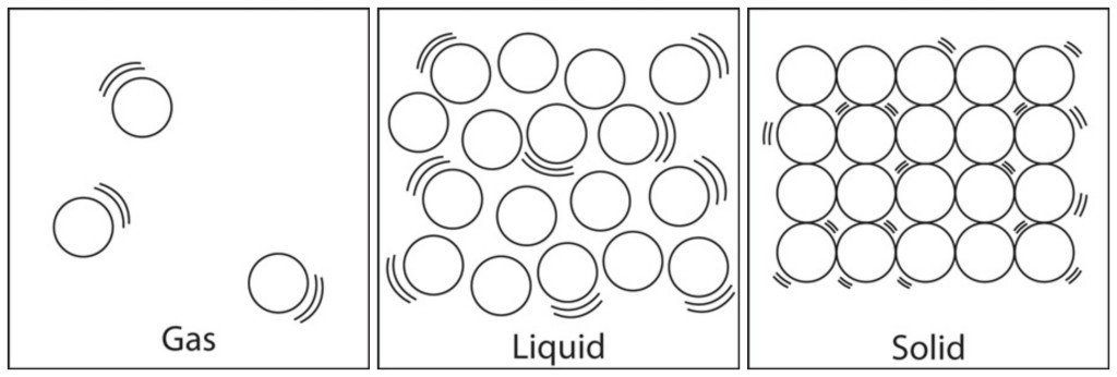
Hello Everyone !!! Hope you all had an amazing week, If you’re in college the new semester probably just started and I hope you’re first few weeks were awesome, I just started grad school and my week was pretty good :). Now moving on with my post, this will be a continuation from my previous post ‘Simulation of Hard Disks - Part 1’ where I tackled this very same problem using Newtonian deterministic mechanics. Ok, so if this is the first time you’re hearing the word Hard disks I do suggest reading my first post where I explain the terms and the rationale behind simulations of this sort.
In my last post I ended on a note that suggested the previous simulation technique has some limitations. So today I’ll start from there, the entire point of simulating hard disks is to predict the behavior of particle systems that we might find in the real world. However such systems have more than 4 particles, and in the previous technique we had to solve the equations of motion for the entire system for every step. While this was possible for 4 particles it would be ridiculously time consuming for a system with 1,000,000s of particles. That in itself is the flaw with this method. This exponential increase in computational complexity drove many scientists to find better ways of simulating hard disk problems.
So the questions is, what is this better way to simulate hard disks? that’s what todays post is all about.
Simulating hard disks using direct sampling
As per the title the simulations I will be presenting today are based on a technique called ‘direct sampling’ which is an interesting concept which stems from the idea of randomness. So what is this direct sampling?
In a nutshell, direct sampling is sort of like randomly picking an apple from a basket of apples and hoping its ripe. However, note that the ripeness of apples will vary according to some distribution(Uniform, Poisson,…). The interesting thing here being there is always some probability that an apple we picked is ripe, so sometimes we might get a good one sometimes we might not luck out.
This idea of using randomness is a corner stone of modern day statistical mechanics. The gif below shows the output from the simulation technique I’ll be discussing today.
If you look closely at the gif above, you would notice a clear difference with respect to the earlier technique. In Newtonian mechanics the simulation revolves with time which means that some state i is directly dependent on its previous i-1 state. So in a gif it looks as if the particles are moving and colliding in real time. However, in this case the the gif just shows different configurations(or samples) of some state that could occur at any time. To explain it in a different way, all the samples you see in the gif above are configurations that the disks could take at some point in time(we don’t know when) that are valid.
So what does it mean to have a valid configuration?A valid configuration, is some placement of the disks within the boundary of the box that doesn’t overlap with each other.
So basically, the gif above just shows some set of legal configurations that the disks could take, it doesn’t necessarily show how the system evolves with time. This is both good and bad. The surprising thing about random sampling is that in terms of simulating hard disks, its possible to replicate the same results we observed from running simulations using Newtonian Mechanics. Before I go into detail about that, first I’ll go through the code for this technique.
The Code
I’ll be demonstrating this technique using Matlab, and unlike the previous method this does not require the use of functions. Since the simulation contains only 4 disks, there can be only 4 possibilities for wall-disk collisions and 6 possibilities for disk-disk collisions as per the table below.
| Disk type A | Disk Type B | Number of collisions |
|---|---|---|
| 1 | 2, 3, 4 | 3 |
| 2 | 3, 4 | 2 |
| 3 | 4 | 1 |
| Total No.of collisions | 6 |
Within the code snippet below, the first few lines of the code determine the initial conditions such as the radius, number of disks, their respective locations and the set of possible collisions of all the disks (which is 6 disk-disk collision pairs & 4 wall-disk collision pairs). Afterwards for a given number of iterations(defined by n) a loop is run for each sample state where each turn 4 random locations for the disks are computed such that the minimum distance between any two disks is greater than the diameter of a disk. This condition ensures that no two disks overlap with each other.
The step for the simulation is not increased until this condition is met, say for an example if the 100th iteration computes an invalid configuration where an overlap is only present between the 1st & 3rd disks where as the 2nd & 4th disks are valid; even then the entire set is rejected resulting in the sample space being completely erased. This form of rejections are called the tabula rasa rejections. These continues rejections occur until a valid set of configurations are obtained, only then would the iteration count be increased from 100 to 101.
clc;
clear;
N=4;
radius=0.15;
diamtr=2*radius;
b=1-radius;
a=radius;
dx=zeros(4,1);
dy=zeros(4,1);
d=zeros(4,2,100);
wall = [1 1; 1 2; 2 1; 2 2; 3 1; 3 2; 4 1; 4 2];
pair = [1 2; 1 3; 1 4; 2 3; 2 4; 3 4];
n=1000000;%number of samples
count =0;
distanceVals=zeros(1,6);

while count < n
	%------positions for disks -----------------------
        for i=1:N
            dx(i)=(b-a).*rand+a;
            dy(i)=(b-a).*rand+a;
            d(i,1,count+1)=dx(i);
            d(i,2,count+1)=dy(i);
        end;

        for i=1:6
            dxa=d(pair(i,1),1,count+1);
            dya=d(pair(i,1),2,count+1);
            dxb=d(pair(i,2),1,count+1);
            dyb=d(pair(i,2),2,count+1);
            distanceVals(i)= sqrt((dxa-dxb).^2+(dya-dyb).^2);
        end;

        if min(distanceVals) >= diamtr
            count=count+1;
    	end
end
The Results
The biggest question you’d probably have after reading thus far about this technique would be How could this even work?. Which is a completely reasonable question, because in Newtonian mechanics the actual equations of motion were computed. Therefore, within the classical boundary the simulation replicates particle motion.
However, here in simple terms all we do is randomly place the particles in a given space for some number of rounds and then bin their locations and now supposedly I say it shows the same behavior as the previous case. The graphs below show a comparison between the histograms for the disk locations for simulations run using Newtonian mechanics and direct sampling for disks 1 & 2(disks 3 & 4 show the same behavior).
01) histogram of X & Y coordinates for disk 1 (MD-Molecular Dynamics, Direct- direct sampling) 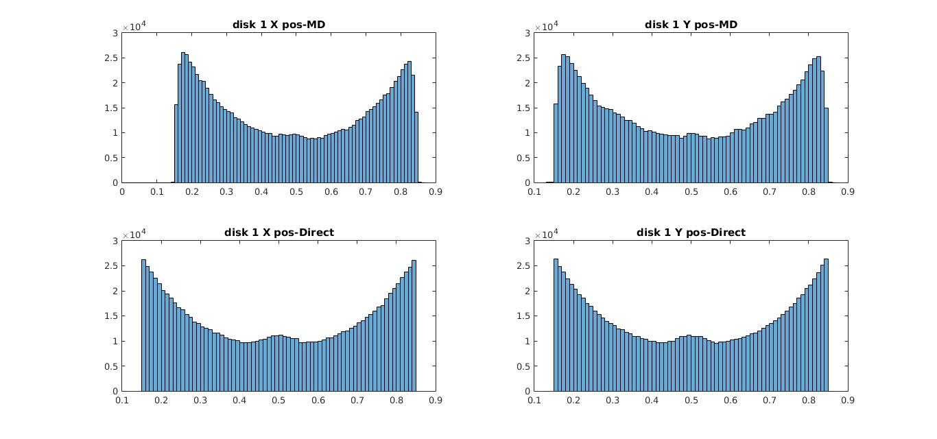
02) histogram of X & Y coordinates for disk 2 (MD-Molecular Dynamics, Direct- direct sampling) 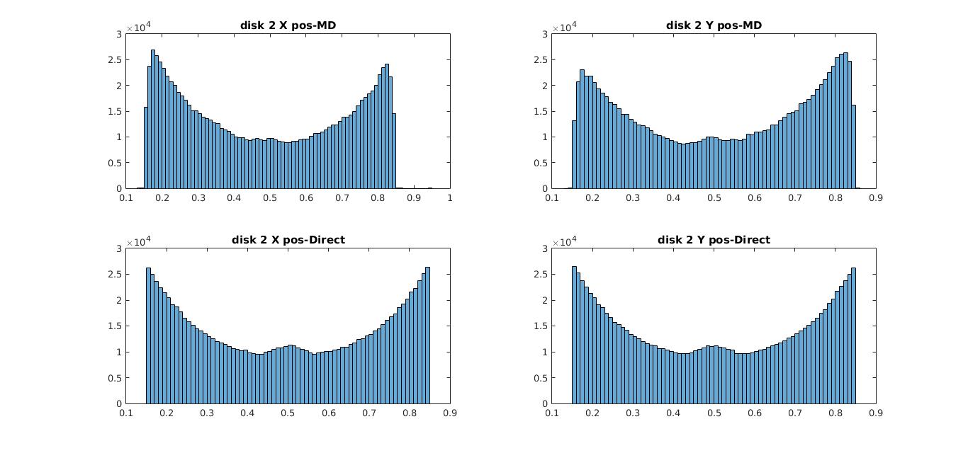
The position distributions show the same behavior where the disks seem to be more attracted towards the edges. As I explained in my previous post the reason behind this phenomena is primarily due to an entropic interaction where at each instance the disks individually try to make more room for the others. The interesting thing here is that even without resorting to complex computations, behavior of complex systems could be replicated using this idea of randomness. However this technique does have its own limitations.
Since the simulation doesn’t evolve with time this technique alone is not sufficient to obtain any idea about how the velocities of the disks vary unlike in the previous case where we saw a Boltzmann distribution for the velocities. Even amidst this, the significant improvement with regards to reducing the computational complexity is very attractive specifically when considering systems with millions of particles. So with that being said I’ll end my post here hoping you all have a newfound appreciation for the power of randomness. (At least in the realm of scientific computing)
So until next time,
Cheers!
Next: From Computational Physics to Computer Science
Prev: Simulation of Hard Disks : Part 1