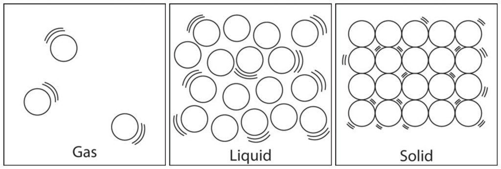
Hey guys !!! Hope all of you are doing great :), In todays post I’ll be demonstrating a very interesting problem of simulating the behavior of hard disks. Now first of all what are hard disks? and why is this even important? We all know that matter around us are either solid,liquid or gaseous. All of these states are some combination of particles, without going in too deep we can simply assume these particles are like spheres in 3-dimensions.
Imagine you suddenly found out some new gas, or liquid and you have it in some container, but you don’t know any of its properties maybe except its mass or the current room temperature. Now how can you predict what will happen when the temperature changes? or when the the number of particles increase? will it become a liquid or become a solid straight away? Those days these sort of problems required experimentation, but now since we have computers we can run simulations and predict their behavior.
Today I’ll be demonstrating something along these lines. Imagine you have a container filed with some gas, and you want to know the behavior of it. By behavior I mean what sort of distribution would the velocities & positions of each particle take? Is there some pattern Or is it completely random?
As it’s with any simulation I’ll start with the assumptions first.
Assumptions
- It’s assumed that the temperature,pressure and volume are constant for the entire duration of the simulation. Therefore any change in particle velocity or position would be only because of some collision.
- The simulation will only have 4 particles, each a 2-D hard disk. A 2-D space inclusive of only 4 particles are considered purely to reduce the computational complexity of the simulation, which you probably will understand when we get into the code. As for the
hard contactpart, this means that the collisions are not damped. - Here instantaneous pair collisions conserve momentum, and wall collisions simply reverse one velocity component. Furthermore, between collisions disks move in a straight line just like a free particle.
Simulating hard disks with Newtonian deterministic mechanics
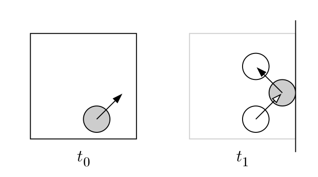
In order to numerically solve the equations of motion for all disks, from a given initial condition we need to propagate all disks up to a next collision in the whole system.Then calculate the new velocities of the collided disks and then continue this process until we decide to stop. Ive coded this simulation using Matlab and used functions extensively. If you’re new to matlab functions click here for a quick introduction.
For a given instance in time there can be a couple of scenarios when it comes to collisions.
- There might be no collisions between disks.
- A disk might collide with a wall.
- Two disks might collide with each-other.
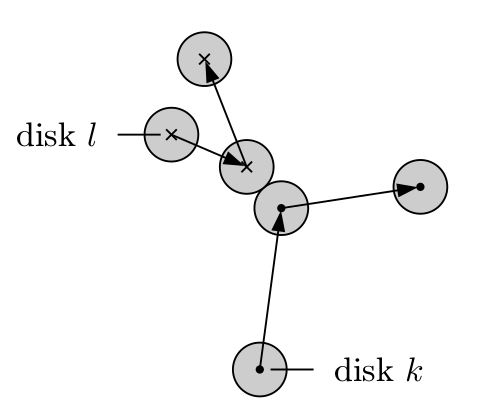
For a case where a collision does not occur the state of the system would not change, all the disks would move along a straight line until it collides with a wall or another disk. When it comes to the simulation, the main task is to identify what type of collision happens first (disk-disk or disk-wall) and between what pair (in our case we have 4 disks). Therefore in the first step two separate functions were defined to calculate the time for all possible disk-disk and disk-wall collisions. Afterwards the min() was taken from all those time values as the next time step when the state of the system changes.
Case 1 : A disk collides with a wall
This case is fairly simple. As per the code snippet below the time for a possible collision is computed based on three cases. In this simulation I’ve considered that a side of the boundary is of unit 1.0 so the coordinates in either x or y directions would be between 0 and 1.0 where as a wall is defined when either x or y is 0 or 1 respectively.
function  t= wallTime(pos,vel,radius)
	if vel > 0
		t= (1.0-radius-pos)/vel;
	elseif vel< 0
		t= (pos-radius)/abs(vel);
	else
		t=double(inf);
	end
The first two cases determine the wall side which the disk would collide in if it traversed without any change. Afterwards depending on the movement direction the time taken until a collision would occur is calculated and returned.
Case 2 : A disk collides with another disk
Now this situation is fairly tricky. Because the number of possible types of collisions that could happen depend on the number of disks. Now its true for the previous case as well. However since we took the sample space as 2-D a given disk could only have one of four collisions since there are only four walls. Since we took only four disks in our sample there are only 6 types of disk-disk collisions. The table below illustrates the possibilities.
| Disk type A | Disk Type B | Number of collisions |
|---|---|---|
| 1 | 2, 3, 4 | 3 |
| 2 | 3, 4 | 2 |
| 3 | 4 | 1 |
| Total No.of collisions | 6 |
Here a collision between disk 1 & 2 or a collision between disk 2 & 1 are considered the same. Therefore for 4 disks there are only 6 possibilities as shown above. What we do here is we compute the time for all the collisions and use that set to find the first pair collision. As per the code below, a collision occurs between two disks when the norm of the spatial distance vector equals twice the radius of a disk.
function t=pairTime(posa,vela,posb,velb,radius)
  delx=[posa(1)-posb(1),posa(2)-posb(2)];
  delxSq=delx(1)^2+delx(2)^2;
  delv=[vela(1)-velb(1),vela(2)-velb(2)];
  delvSq=delv(1)^2+delv(2)^2;
  scalar=delv(1)*delx(1)+delv(2)*delx(2);
  Up=scalar^2-delvSq*(delxSq-4*radius^2);
  if Up> 0.0 && scalar < 0.0
  		t= -(scalar+sqrt(Up)) / delvSq;
  	else
  		t=double(inf);
  	end
Computing the time until the next event
The code below combines the two functions I described above in order to find the next collision event. The objective of this simulation is to record the state of a system for a given time period. And we know now the state of a system changes when a disk collides with a wall or another disk. The code below explains how the above two functions are combined together to find the time when the next event occurs.
function [t,minWallTime,minPairTime,t_wall,t_pair] = nextCollisionTime(POS,VEL,radius)
	wall=[1 1; 1 2; 2 1 ; 2 2 ; 3 1 ; 3 2 ; 4 1 ; 4 2];%1->wall 1(0) ,2->wall 2(1)
	pair=[1 2 ; 1 3; 1 4; 2 3 ; 2 4 ; 3 4];
	t_wall=zeros(1,8);
	t_pair=zeros(1,6);
	count=1;
	%wall collision-----------------------
	for k=1:4
		for l=1:2
			posTemp=POS(k,l);
			velTemp=VEL(k,l);
			t_wall(count)=wallTime(posTemp,velTemp,radius);
			count=count+1;
		end
	end
	minWallTime=min(t_wall);
	%pair collision-----------------------
	for i=1:6
		pos1=POS(pair(i,1),:);
		vel1=VEL(pair(i,1),:);
		pos2=POS(pair(i,2),:);
		vel2=VEL(pair(i,2),:);
		t_pair(i)=pairTime(pos1,vel1,pos2,vel2,radius);
	end
	minPairTime=min(t_pair);
	t=min(minPairTime,minWallTime);
Running the simulation
So intuitively this is how the program collects data. Say the simulations starts at time t=0 and it’s supposed to collect data every 0.10 seconds. The first thing to do is calculate the time for the next event. Using the function above. In our case we get that the next event occurs at t=0.15 seconds. In such a case the program will iterate a step to 0.10 seconds and then compute the new positions of the disks(Note that the velocities wont change) afterwards the new velocities & positions at 0.15s will be computed. Because we already found out that a collision will occur at this time step. These new velocities and positions will be again used at the next iteration at 0.20s not the ones before. This process needs to iterate until we have enough samples for our data set.
clc;
clear;

intialPos=[0.25 0.25; 0.75 0.25; 0.75 0.75; 0.25 0.75];%intial posiitons of the disks
initalVel=zeros(4,2);
for i=1:4; %setting up initial velocities
	initalVel(i,1)=2*rand-1;
	initalVel(i,2)=2*rand-1;
end
%----definiing collision types--------
wall=[1 1; 1 2; 2 1 ; 2 2 ; 3 1 ; 3 2 ; 4 1 ; 4 2];%1->wall 1(0) ,2->wall 2(1)
pair=[1 2 ; 1 3; 1 4; 2 3 ; 2 4 ; 3 4];
radius=0.15 ;%radius
t=0.0;%initial time
dt=0.01;%time step
n=1000000;%number of samples
time=zeros(1,n);
time(1)=t;
nextColtime=0;

wt=zeros(1,8);%wall times calculated per collision
pt=zeros(1,6);%pair collisions times per collision

pos=zeros(4,2,n);
pos(:,:,1)=intialPos;
vel=zeros(4,2,n);
vel(:,:,1)=initalVel;

%----calculating next collision event----------------
count =1;
POS=intialPos;
VEL=initalVel;
[tmin,minWallTime,minPairTime,allWallTime,allPairTime]=nextCollisionTime(POS,VEL,radius);
%----------------------------------------------------
while count <= n
	t=t+dt;
	if t < tmin
		time(count+1)=t;
		vel(:,:,count+1)=vel(:,:,count);
		for i=1:4
			pos(i,1,count+1)=pos(i,1,count)+dt*vel(i,1,count);
			pos(i,2,count+1)=pos(i,2,count)+dt*vel(i,2,count);
		end
	else
		time(count+1)=tmin;
		vel(:,:,count+1)=vel(:,:,count);
		for i=1:4
			pos(i,1,count+1)=pos(i,1,count)+(tmin-t-dt)*vel(i,1,count);
			pos(i,2,count+1)=pos(i,2,count)+(tmin-t-dt)*vel(i,2,count);
		end
		if minWallTime < minPairTime
			[Lia,Locb]=ismember(minWallTime,allWallTime);
			collision = single(wall(Locb,1));
			direction = single(wall(Locb,2));
			vel(collision,direction,count+1)=vel(collision,direction,count+1)*(-1.0);
		else
			[Lia,Locb]=ismember(minPairTime,allPairTime);
			a=pair(Locb,1);
			b=pair(Locb,2);
			delx=[pos(b,1,count+1)-pos(a,1,count+1),pos(b,2,count+1)-pos(a,2,count+1)];
			absx=sqrt(delx(1)^2+delx(2)^2);
			ePerp=delx/absx;
			delv=[vel(b,1,count+1)-vel(a,1,count+1),vel(b,2,count+1)-vel(a,2,count+1)];
			scalar=delv(1)*ePerp(1)+delv(2)*ePerp(2);
			for k=1:2
				vel(a,k,count+1)=vel(a,k,count+1)+ePerp(k)*scalar;
				vel(b,k,count+1)=vel(b,k,count+1)-ePerp(k)*scalar;
			end
		end
		t=tmin;
		POS=pos(:,:,count+1);
		VEL=vel(:,:,count+1);
		[Newtmin,minWallTime,minPairTime,allWallTime,allPairTime]=nextCollisionTime(POS,VEL,radius);
		tmin=tmin+Newtmin;
	end
	count=count+1;
end
From this point on you can either decide to draw the disks at each time step which will give a nice graphical output like in the gif above Or more importantly you can visualize the position and velocity data of these disks(particles).
The Results
First, lets look at the position data for all the disks. The histograms below represent the binned values for the x coordinate positions & the y coordinate positions for all 4 disks respectively.
histogram of x coordinates for all disks 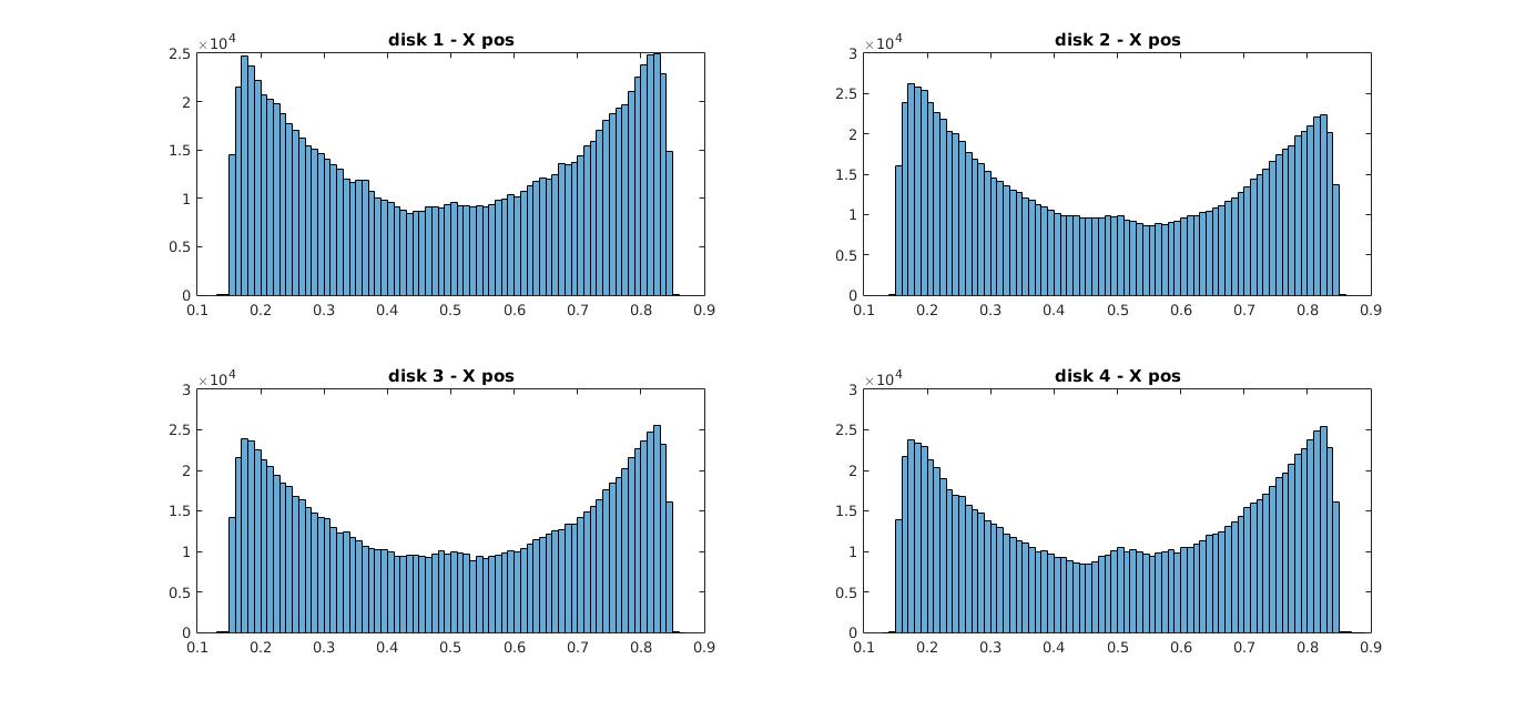
histogram for y coordinates for all disks 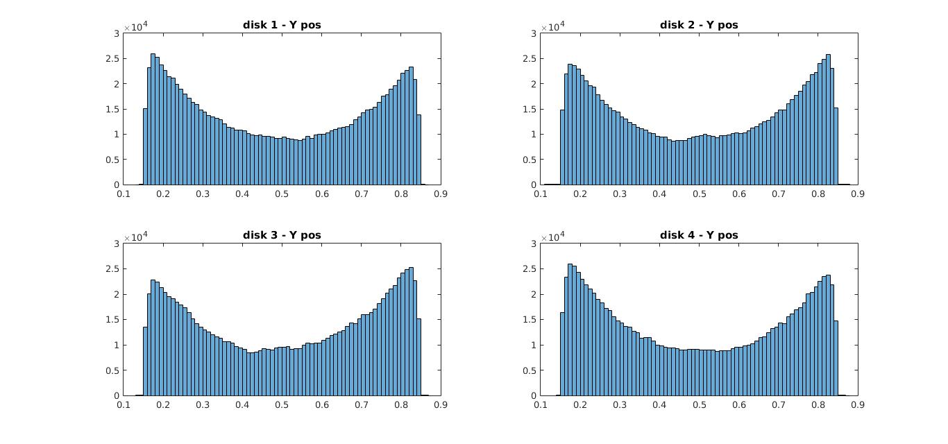
Now usually you’d expect the histogram to have peaks at the middle between 0 & 1 because particles when in the middle have more room to spread out, but the observation here is the opposite. The disks seem to be near the edges/walls more than at the middle.
why does this happen ?
an interesting question. This phenomena is explained using findings from Asakura & Osawa but I wont go in-depth about that here, instead let me explain it simply.
The reason for this unusual behavior is this, now lets say at some given moment disk 1 is at some edge(near a wall) then the region(area) that the other disks could move in without a collision is much larger than when disk 1 would be in the middle. Therefore increasing the ability of the other disks to move freely without a collision.(In other words it increases the entropy of the entire system). Likewise all the disks try to move closer to the edges so as to free more space for the others. Because the disks like to have as much free space to move for themselves.
This is the reason you see a histogram like this. I’ll go in detail into this phenomena in a future post with more mathematical rigor :), so this explanation will have to do for now.
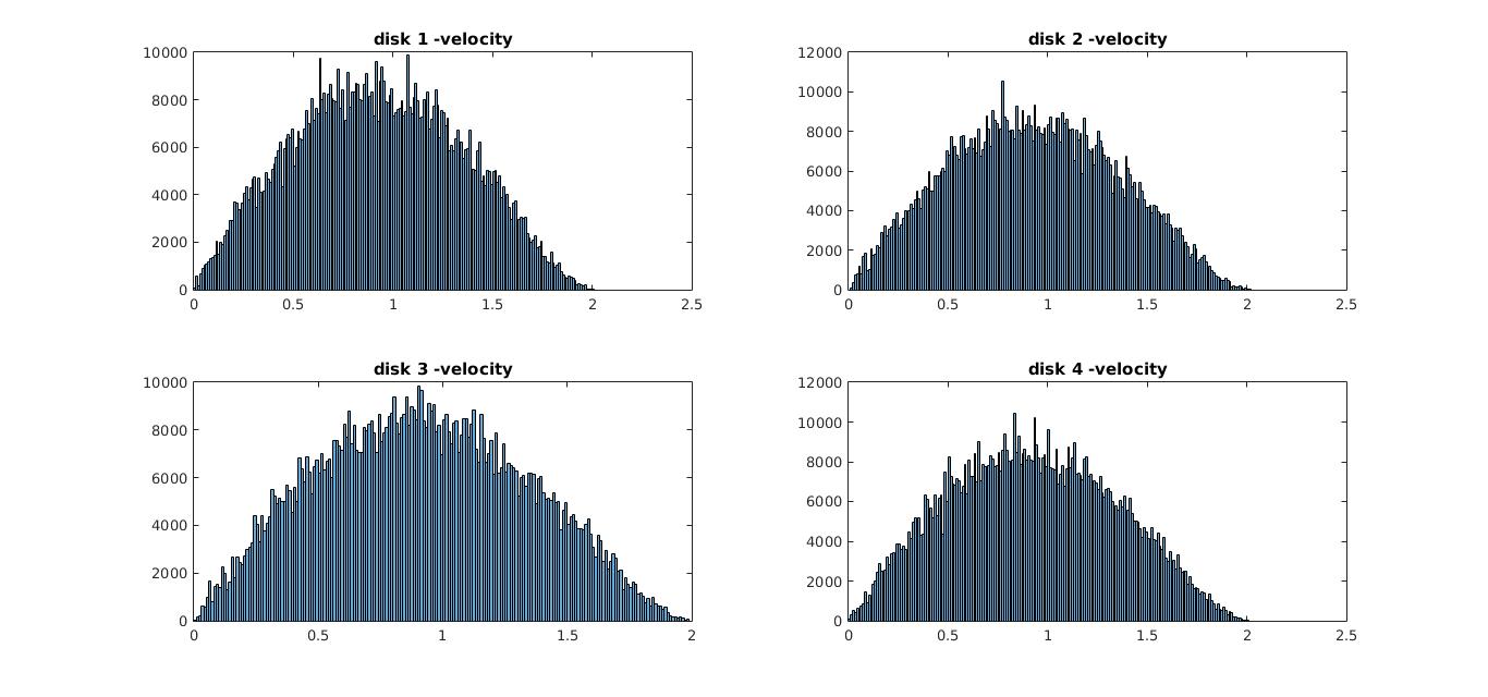
Now if you look at the velocity distribution below you’ll see it’s in fact a Boltzmann distribution which is pretty close to how velocities get distributed for particles(like gases) in a box. So there is in fact some pattern to the particle behavior within the classical limits we defined.
I know the code was a bit complex here, but this goes to show that simulations can in fact be used to predict behavior of matter. However there are some limitations in this method. Don’t worry, I wont explain it here and make this post any longer, instead I’ll talk about them in my next post and show an easier method to simulate this very same problem with half the code.
So until next time,
Cheers!
Next: Simulation of Hard Disks : Part 2
Prev: Image processing with Matlab: Combining video-game sprites